
The understanding of the flow of fluids, which include gases, liquids, and others, has been a prominent field of study for centuries. In 2022, we had the 200th anniversary of the first appearance of the Navier-Stokes equations in the literature, introduced by Claude-Louis Navier in 1822. Initially, it was considered that there was no viscosity until Navier brought this concept to light, considering the resistance in the fluid due to the molecules' interactions with one another under the influence of various forces. Previously, fluid motion was often studied under the assumption of no viscosity, which made the mathematics easier but the physics unrealistic. Stokes later on appears in the scene by reformulating the equation in late 1840s, by continuous fluid assumption. The work eventually turns up in forms of equations to define the velocity, pressure, and how various factors are affecting the fluid flow, basically representing Newton’s first law.
There were a few exact, analytical solutions derived on the way by many researchers for some highly idealised flows, such as Plane Poiseuille flow, Hagen–Poiseuille flow, Couette flow, Rayleigh Flow, Taylor-Green vortex, and Blasius boundary layer solution. But soon, they started to notice, in three dimensions, no one could prove that these equations always have smooth, well-behaved solutions. In 2000, this concern became famous when the Clay Mathematics Institute listed the Navier–Stokes existence and smoothness problem as one of its Millennium Prize Problems, offering one million dollars for a proof. More than two decades have passed, and the prize remains unclaimed. The equations work extraordinarily well while in practice, but have baffled mathematicians across to prove the existence of the smooth solutions.
We just don’t have such ideal geometries and boundary conditions in real life that we rely on the derived analytical solutions. We have some very complex geometries and problem definitions, so how do we exactly reach the final, at least expected solution? So, we start relying on the numerical methods to solve these differential equations through various methods, focusing more on the numbers than the formulas. This is what we know as Computational Fluid Dynamics or more commonly as CFD. In CFD, the flow domain is divided into a large number of small control volumes or grid points. The Navier–Stokes equations are then rewritten in a discrete form and solved step by step on a computer.
Each problem statement would require a different numerical method, a different algorithm, varying computational time and accuracy. But for all, the time step taken is very minimal, where the pressure and velocity fields are iterated until they reach convergence, initially decided by a tolerance level. Through these techniques, we don’t get the exact solution, but more of an approximation.
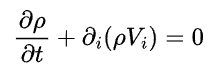
Let’s first take a look at the Navier-Stokes equation, which includes the continuity equation and the directional momentum equations.

These equations are more like written considering various assumptions and later are discretised using various schemes, and are computationally modelled by choosing a proper time-scheme, discretisation technique, algorithms and much more to consider.
The governing differential equations are partial differential equations, which, upon discretisation, are turned into finite difference or finite volume equations. Ensuring the stability of these can result in approximate solutions of the FDEs. And further reaching the convergence (Δx, Δt→0) would result in exact solution of the partial differential equation. Also, ensuring the consistency of FDEs, as (Δx, Δt→0), brings us back to the governing partial differential equations.
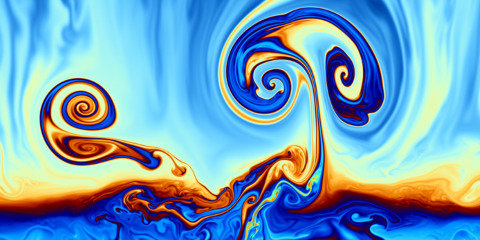
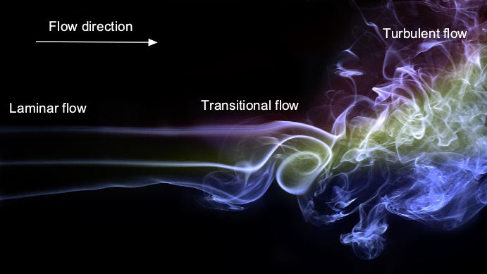
There are various models and theories developed for the case of turbulent flow. Laminar flows are so simpler to understand due to their unrealistic but ideal nature. While turbulence is what we always encounter. Turbulence has a beauty in itself. It can be thought of as a Mandelbrot set, which is like a fractal set. The fractal repeats its appearance again and again, upon zooming in, and if you lose track of where you zoomed, you may never know exactly what part you were looking at. In a similar way, turbulence involves the continuous formation of eddies and vortices. As we move to smaller and smaller scales, new eddies continue to appear, making turbulence inherently complex, complicated, and more chaotic.
But it isn’t that we can’t replicate this complex behaviour. Actually, we can, as is called as direct numerical simulation. In DNS, the Navier–Stokes equations are solved directly without any turbulence models, resolving all the eddies, and literally all of them, from the largest flow structures down to the smallest dissipative scales. In theory, this gives the most accurate description of a turbulent flow. In practice, however, DNS is extremely expensive because of the extreme fine mesh size and timesteps, making it more impractical for most real-world engineering flows. Let’s say, we don’t want to waste our time and money on all the vortices, so that’s where the Large Eddy Simulation or LES for short, comes in.
LES takes a middle path between accuracy and cost. Instead of resolving all turbulent scales, LES resolves the large, high-energy eddies and models only the smaller ones. Since the largest eddies depend strongly on geometry and flow conditions, LES captures more than simpler models, while remaining far less expensive than DNS. This makes LES attractive for unsteady flows where detailed turbulence structure matters. In practical terms, we use what’s known as RANS, or Reynolds-Averaged Navier–Stokes. In RANS, the equations are time-averaged, and the effects of all turbulent fluctuations are modelled rather than resolved. This makes RANS computationally efficient and more often used in the industry.
From an Engineering point of view, the DNS, LES, RANS, and so many other methods yield results sufficient for further analysis, but from a mathematical point of view, however, something fundamental is still missing. We do not know whether these equations always behave nicely in three dimensions, or whether they can develop singularities in finite time.
The million-dollar prize, thus, is about understanding whether the equations that describe fluid motion are complete at the most basic level. A proof would tell us whether turbulence is merely complex or whether the equations themselves have some hidden treasure in them. Thus, the wait from decades will continue, and the proof will still remain unanswered as the equations will stay in their unusual position. These are used and trusted by the engineers, challenged by mathematicians and always followed by nature. Perhaps that is why the prize remains unclaimed, not because the equations fail eventually, but because they reveal how much there is still to learn about something as simple as flowing water.