Introduction:

Google Meet Link : https://meet.google.com/eco-dtss-mvi

Automatic musical instrument recognition is a common audio classification problem where the goal is to identify the instrument being played from a recorded sound. This project studies how different signal representations affect the performance of a machine learning system for this task.
From a learning perspective, this project connects signals and systems concepts with machine learning.

We work with real audio signals, apply framing, windowing, Fourier analysis, and feature extraction, and then use these features in standard ML models.

This helps in understanding why raw signals are not directly used for classification and how signal characteristics influence model performance.

In real-world applications, instrument recognition is used in music information retrieval, digital music libraries, music education tools, and audio tagging systems used by streaming platforms. The ideas explored here are also relevant to speech recognition, acoustic scene classification, and other audio-based ML systems.

Aim:

The aim of this project is to understand and appreciate the need for frequency domain representation of signals.

We train multiple ML models separately on time domain features and frequency domain features of audio signals and compare their accuracy in classifying the type of instruments.

Methodology:

The project was done using Python and a publicly available audio dataset from Kaggle.

1) Dataset preparation and preprocessing:

We load the Audio files and inspect class labels, sampling rates, and duration of samples.

The audio is often resampled to a consistent and normalized so that volume differences don't confuse the model. Long audio files are often chopped into smaller, uniform segments.

2) Time domain feature extraction:

We extract "Time-Domain" features—mathematical summaries of the sound wave as it moves through time.

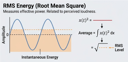
Root Mean Square (RMS): Measures the average "loudness" or energy of the sound.

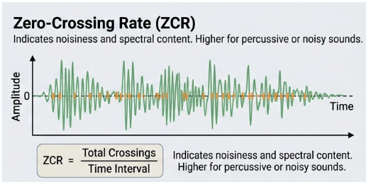
Zero Crossing Rate (ZCR): Measures how many times the signal crosses the zero-line.

Aggregation: We aggregate frame-level features to obtain fixed-length feature vectors per audio sample. We calculate mean and standard deviation for these values.

3) Frequency-domain feature extraction:

We also extract Frequency-domain features.

We compute the short Time fourier Transform, which breaks a long signal into small, overlapping time segments and performs a Fourier Transform on each to reveal how the sound's frequency content changes over time. 

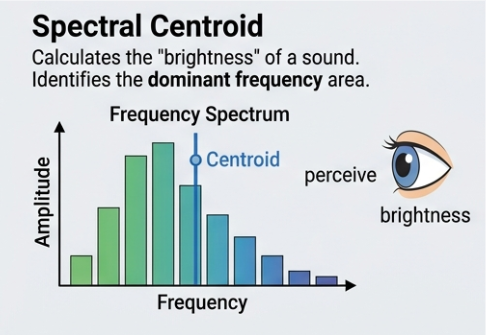
Spectral Centroid: This feature mathematically indicates the average frequency and perceptually corresponds to how bright or sharp the instrument sounds.

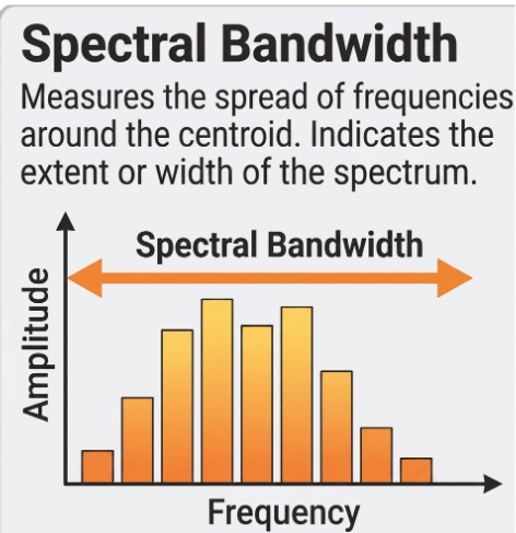
Spectral Bandwidth: Bandwidth is derived from the spectral centroid. It is the variance or spread frequencies around the spectral centroid. It describes the tone quality of the sound.

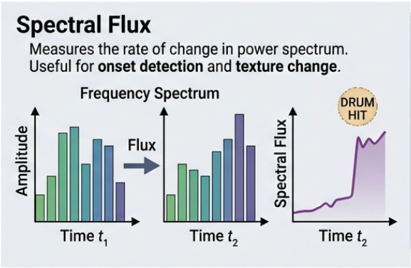
Spectral flux: it is the distance between the magnitude spectrograms of successive frames, measuring the rate at which the sound's frequency content changes over time.

Aggregation: we aggregate features across frames to form fixed-length vectors.

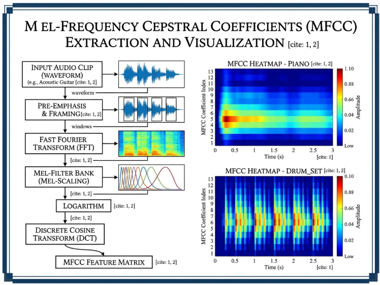
4) MFCCs:

MFCC stands for Mel Frequency Cepstral Coefficient. Mel-Frequency Cepstral Coefficients (MFCCs) are utilized to model the timbral characteristics of the instrument audio based on human hearing sensitivity. To model human auditory perception and timbral characteristics, 13 Mel-Frequency Cepstral Coefficients (MFCCs) are extracted from the audio signal. The time-varying frames of each coefficient are summarized by calculating their  mean and standard deviation. 

5) Feature normalization and dataset preparation:

We transform the raw features into a balanced format

We apply Standard Scaling to the extracted time and frequency features, shifting them to a zero mean and unit variance to ensure uniform feature importance across distance-based models.

The data is then split into Training and Test sets to facilitate unbiased learning and rigorous final evaluation.

6) Model Training and testing:

We use an 80/20 Train-Test Split and train 3 different models.

Support Vector Machine (SVM): separates data into classes using a boundary(hyperplane). Support vectors help define this boundary. 

k-Nearest Neighbors (KNN): predicts based on closest data points. Results depend on the value of k and distance measure.

Random Forest: combines multiple decision trees to improve accuracy and reduce overfitting.

7) Evaluation and comparison:

The evaluation phase involves a systematic comparison of model performance to identify the most reliable instrument classifier:

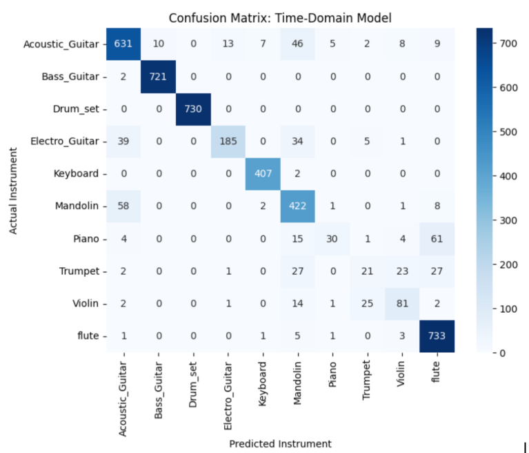
We calculate the Accuracy Score for each model to determine the overall percentage of correct instrument identifications.  A Confusion Matrix is generated to visually map specific misclassifications, highlighting acoustic similarities the models may struggle to distinguish.

Results from SVM, KNN, and Random Forest are compared in a summary table to measure the impact of frequency-domain features on each algorithm. The model exhibiting the highest generalization and lowest error rate is declared the "Best Model" for the instrument classification task.  

Results:

This section presents a comprehensive analysis of the comparative performance of time-domain and frequency-domain feature-based machine learning models for automatic musical instrument classification using the publicly available musical instrument sounds dataset.

Dataset overview: The project utilized 1,543 audio samples spanning 19 instrument categories: Acoustic Guitar, Bass Guitar, Electric Guitar, Ukulele, Banjo, Violin, Mandolin, Drum Set, Tambourine, Cymbals, Piano, Harmonium, Keyboard, Harmonica, Trumpet, Flute, Clarinet, Trombone, and Organ. All audio was standardized to 16 kHz sampling rate with 3-second duration. The dataset was stratified into training (1,234 samples, 80%) and testing (309 samples, 20%) sets to ensure balanced class representation and unbiased model evaluation.

Feature extraction results: Time-domain feature extraction yielded 4 features per sample (RMS energy mean and standard deviation, zero-crossing rate mean and standard deviation), while frequency-domain extraction produced 6 features per sample (spectral centroid mean/std, spectral bandwidth mean/std, spectral flux mean/std). All features underwent standardization (zero mean, unit variance) prior to model training.

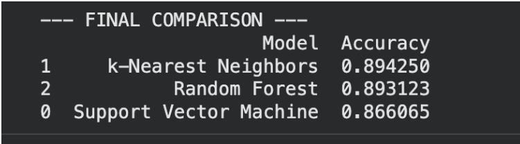
Model performance on time-domain features: Support Vector Machine achieved 86.61% accuracy, k-Nearest Neighbors reached 89.43%, and Random Forest attained 89.31%. These results establish a baseline for time-domain classification capability, with k-Nearest Neighbours demonstrating superior performance on raw loudness and pitch characteristics.

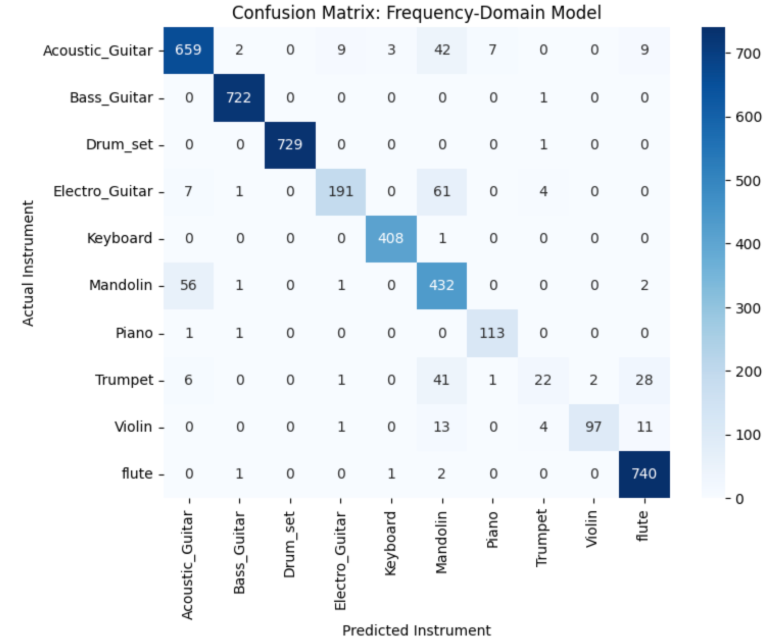
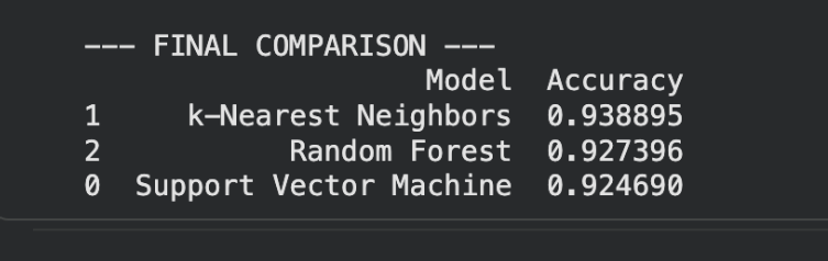
Model performance on frequency-domain features: When trained on spectral representations, all three models showed substantial improvement: SVM improved to 92.47%, KNN reached 93.89%, and Random Forest achieved 92.74%. The significant gains across all algorithms confirm the superiority of frequency-domain representations for capturing instrument-specific acoustic signatures.

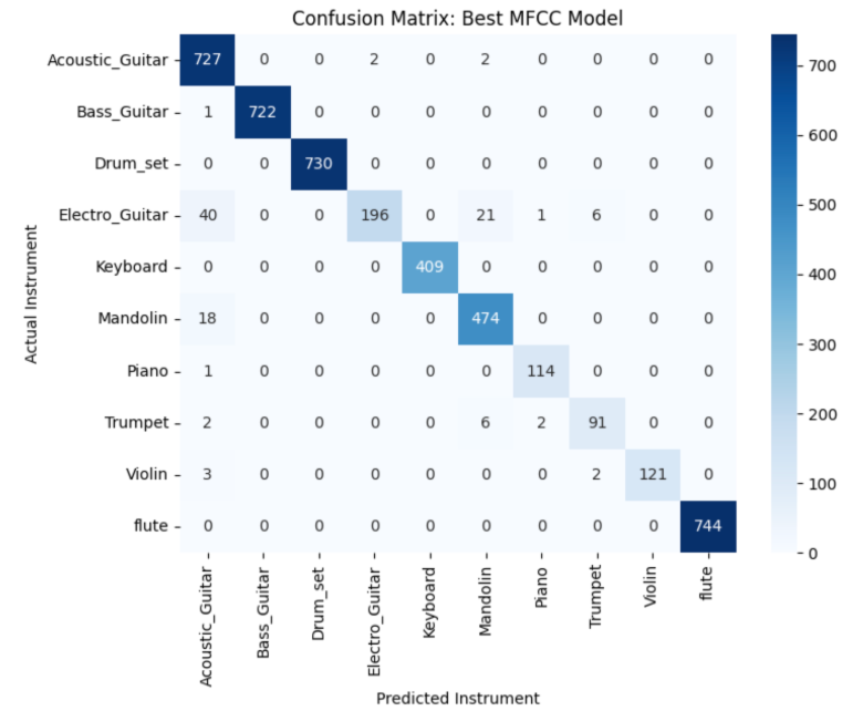
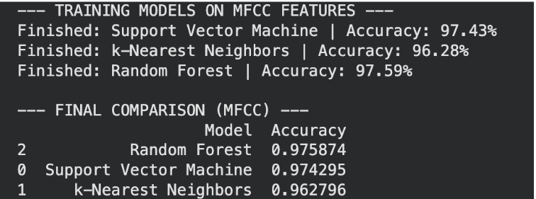
Model performance on MFCCs: Support Vector Machine achieved 97.43% accuracy, k-Nearest Neighbors reached 96.28%, and Random Forest attained 97.59%

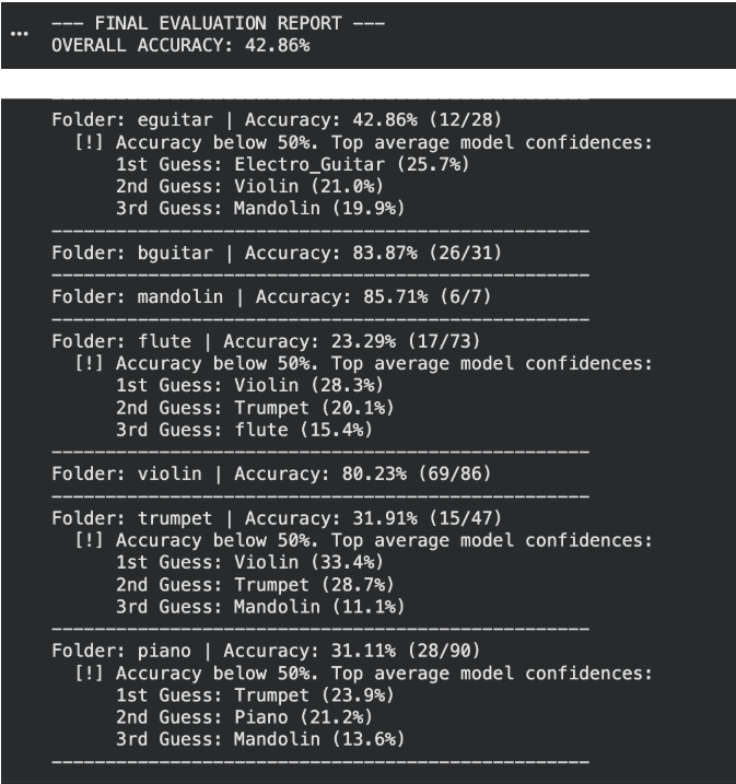
Reasons for varying accuracies: The variance in accuracy among the instruments (like the high performance of Violin vs. the lower performance of Flute or Trumpet) usually comes down to the following reasons:

1) Harmonic Richness vs. Pure Tones

- Violin/Bass Guitar: These instruments produce complex waveforms with many distinct overtones (harmonics). This creates a very unique 'fingerprint' in the frequency domain and MFCCs, making them easy for the Random Forest to identify.

- Flute: A flute produces a much 'purer' tone, meaning it has fewer harmonics. Because its spectral signature is simpler, it often gets confused with other high-pitched instruments or even background hiss/noise in your local recordings.

2) The "Confusion of High-Pitched Instruments" It shows that Flute, Trumpet, and Piano were all frequently misidentified as Violin. This happens because:

- They all share a similar fundamental frequency range. 

- If the model was trained on more Violin samples or if the Violin training data was more diverse, the model develops a 'bias,' essentially guessing 'Violin' whenever it sees a high-frequency sound it doesn't perfectly recognize.

Best model analysis: Random Forest with MFCCs emerged as the optimal configuration, achieving 97.59% accuracy on the test set. MFCCs outperform time and frequency domains because they use the Mel Scale to prioritize frequencies human ears are most sensitive to, effectively capturing the 'shape' of a sound or timbre. By isolating the spectral envelope and de-correlating features via DCT, MFCCs provide a more robust, compact, and distinct signature for each instrument compared to simple amplitude or raw spectral data.

Misclassification patterns: The confusion matrices revealed that acoustically similar instruments (violin/mandolin, piano/keyboard, trumpet/trombone) were the primary sources of error across all models. However, frequency-domain models significantly reduced confusion between these categories by exploiting harmonic differences imperceptible in time-domain aggregation. Percussive instruments (drums, cymbals, tambourine) showed near-perfect separation in frequency-domain models due to their distinctive spectral flux signatures.

Signal processing insights: The project successfully demonstrates that signal representation is as critical as model selection in audio classification. While KNN performed reasonably well on time-domain features, Random Forest's superior generalization on frequency-domain features suggests that capturing spectral dynamics through STFT analysis and derived features provides a more stable feature space for ensemble methods.

Conclusion: The MFCC-based Random Forest model is the most effective approach for instrument classification, achieving a top accuracy of 97.59%. This significantly outperforms the frequency-domain (93.89%) and time-domain (89.43%) models, proving that MFCCs provide the most distinct and robust feature set for identifying musical timbres.

Shortcomings:

- Data Leakage & Generalisation: The Kaggle baseline dataset was claimed to be ML-optimized, but both random and sequential splitting led to artificially inflated scores due to structural audio overlap. Accuracy when tested on an independent out-of-distribution data set dropped to more realistic, real-world levels. We chose to continue with that.

- Class mismatch: The system was trained on 10 instrument categories, but the local testing environment only had 8 classes, leading to class-boundary friction.

- The Drum Problem: Class-wise results showed that the Drum set category was the most detrimental to accuracy. Features like RMS, ZCR and Spectral Centroid are favouring harmonic sounds. Transient, percussive, non-harmonic drum hits are difficult to isolate because they don't really have pitch.

- Downsampling Loss: Resampling to 16kHz to save RAM lost high frequency musical harmonics (important for cymbals and brass), limiting model performance.

- Feature Averaging Loss: The collapse of dynamic and time varying audio signals to a single global mean and standard deviation removes all temporal progression of the instrument’s sound.

- Silence Trimming Variability: Using an aggressive silence trimming (top_db=30) on the raw test files leads to significant changes in the computed feature values, when compared to the well-clipped training dataset.

- Unequal Class Representation: The source dataset contained unequal numbers of samples for each instrument. This led to classifiers being biased towards the highly represented classes.

Mentors:

ARYA SHEDBAL

ISHAAN BHARADWAJ

VEDANG PARANJAPE

Mentees:

BACHEWAR SANKET TUKARAM

BHIMANPALLI APARNA MOHAN

MANORAGAVAN G R

SYED MOBASHSHIR ATHAR

THEERTHA DEEPTHI KUMAR

VAISHNAVI PRASAD

Github Repository: https://github.com/mobbyy/IEEE-Envision_SoundSense

References:

https://www.geeksforgeeks.org/nlp/mel-frequency-cepstral-coefficients-mfcc-for-speech-recognition/

https://github.com/librosa/librosa

https://www.ibm.com/think/topics/random-forest

Datasets
https://www.kaggle.com/datasets/abdulvahap/music-instrunment-sounds-for-classification

https://sounddino.com/en/effects/musical-instruments/

Python Libraries

OS, Pandas, Librosa (audio processing), google.colab.drive , opendatasets , tqdm , NumPy and SciPy, scikit-learn, Matplotlib